Chapter 3 QR 分解
任何的实方阵都可以做QR分解:
\[A = QR\]
其中 Q 是正交阵, R 是 upper triangle 矩阵.
Q 作为正交矩阵,有很多很好的特性:
- \(QQ^T = I\)
- det(Q) = ±1, 如果 det(Q) = 1 则为旋转变换,说起旋转变换又会想到SO(n) 李群和李代数
- 可以给我们提供一组正交基
3.1 Gram-Schmidt
我们可以通过Gram–Schmidt来计算Q:
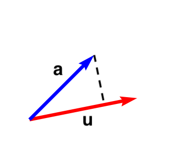
首先定义projection 操作:
\[\operatorname {proj} _{\mathbf {u} }\mathbf {a} ={\frac {\left\langle \mathbf {u} ,\mathbf {a} \right\rangle }{\left\langle \mathbf {u} ,\mathbf {u} \right\rangle }}{\mathbf {u} }\]
也就是把 \(\mathbf{a}\) 投影到 \(\mathbf{u}\) 方向上。
假设 \(A=\left[\mathbf {a} _{1},\ldots ,\mathbf {a} _{n}\right]\), 那么可以找到一组正交基:
\[ \begin{aligned} \mathbf {u} _{1}&=\mathbf {a} _{1},&\mathbf {e} _{1}&={\mathbf {u} _{1} \over \|\mathbf {u} _{1}\|}\\\mathbf {u} _{2}&=\mathbf {a} _{2}-\operatorname {proj} _{\mathbf {u} _{1}}\,\mathbf {a} _{2},&\mathbf {e} _{2}&={\mathbf {u} _{2} \over \|\mathbf {u} _{2}\|}\\\mathbf {u} _{3}&=\mathbf {a} _{3}-\operatorname {proj} _{\mathbf {u} _{1}}\,\mathbf {a} _{3}-\operatorname {proj} _{\mathbf {u} _{2}}\,\mathbf {a} _{3},&\mathbf {e} _{3}&={\mathbf {u} _{3} \over \|\mathbf {u} _{3}\|}\\&\vdots &&\vdots \\\mathbf {u} _{k}&=\mathbf {a} _{k}-\sum _{j=1}^{k-1}\operatorname {proj} _{\mathbf {u} _{j}}\,\mathbf {a} _{k},&\mathbf {e} _{k}&={\mathbf {u} _{k} \over \|\mathbf {u} _{k}\|} \end{aligned} \]
A 可以表示为:
\[ \begin{aligned} \mathbf {a} _{1}&=\langle \mathbf {e} _{1},\mathbf {a} _{1}\rangle \mathbf {e} _{1}\\\mathbf {a} _{2}&=\langle \mathbf {e} _{1},\mathbf {a} _{2}\rangle \mathbf {e} _{1}+\langle \mathbf {e} _{2},\mathbf {a} _{2}\rangle \mathbf {e} _{2}\\\mathbf {a} _{3}&=\langle \mathbf {e} _{1},\mathbf {a} _{3}\rangle \mathbf {e} _{1}+\langle \mathbf {e} _{2},\mathbf {a} _{3}\rangle \mathbf {e} _{2}+\langle \mathbf {e} _{3},\mathbf {a} _{3}\rangle \mathbf {e} _{3}\\&\vdots \\\mathbf {a} _{k}&=\sum _{j=1}^{k}\langle \mathbf {e} _{j},\mathbf {a} _{k}\rangle \mathbf {e} _{j} \end{aligned} \]
所以有:
\[Q=\left[\mathbf {e} _{1},\ldots ,\mathbf {e} _{n}\right]\]
\[ R = \begin{pmatrix}\langle \mathbf {e} _{1},\mathbf {a} _{1}\rangle &\langle \mathbf {e} _{1},\mathbf {a} _{2}\rangle &\langle \mathbf {e} _{1},\mathbf {a} _{3}\rangle &\ldots \\0&\langle \mathbf {e} _{2},\mathbf {a} _{2}\rangle &\langle \mathbf {e} _{2},\mathbf {a} _{3}\rangle &\ldots \\0&0&\langle \mathbf {e} _{3},\mathbf {a} _{3}\rangle &\ldots \\\vdots &\vdots &\vdots &\ddots \end{pmatrix} \]
这个 R 为上三角矩阵由上面的计算过程看起来是一目了然,实际上我们动脑想一想也会觉得很清楚,因为 \(\mathbf{a}_{1}\) 定义了 \(\mathbf{e}_{1}\) ,而 \(\mathbf{a} _{2}\) 则完全由 \(\mathbf{e}_{1}, \mathbf{e}_{2}\) 确定, \(\mathbf{a}_{k}\) 只会由 \(\mathbf{e}_{1} \cdots \mathbf {e}_{k}\) 确定,所以当然就是上三角的。
不过实际上, Gram-Schmidt 计算方式并不是很数值稳定,想象一下矩阵:\(\begin{pmatrix} 1 & 1 + \varepsilon \\ 1 & 1\end{pmatrix}, \varepsilon \ll 1\),其实计算过程可能会出很大的问题。因为除以一个极小的数可能会带来很多无效数据。
3.2 Householder变换
projection 我们也可以写成矩阵形式:
\[\operatorname {proj} _{\mathbf {u} }\mathbf {a} ={\frac {\left\langle \mathbf {u} ,\mathbf {a} \right\rangle }{\left\langle \mathbf {u} ,\mathbf {u} \right\rangle }}{\mathbf {u} }\]
\[ \operatorname {proj} _{\mathbf {u} }\mathbf {a} = {\frac {\mathbf {u}^T \cdot \mathbf {a} }{\mathbf {u}^T \cdot \mathbf {u} }} \cdot {\mathbf {u} } = {\frac { (\mathbf {u}^T \cdot \mathbf {a}) \cdot \mathbf {u} }{\mathbf {u}^T \cdot \mathbf {u} }} \]
点乘复合交换律和结合律,所以我们可以继续写成:
\[ \operatorname {proj} _{\mathbf {u} }\mathbf {a} = {\frac { \mathbf {u}\cdot \mathbf {u}^T \cdot \mathbf {a} }{\mathbf {u}^T \cdot \mathbf {u} }} \]
这里 \(\mathbf {u}\cdot \mathbf {u}^T\) 是一个 3 x 3 的矩阵,所以
\[ P = {\frac { \mathbf {u}\cdot \mathbf {u}^T }{\mathbf {u}^T \cdot \mathbf {u} }} \]
又称作投影的矩阵形式。它本身也有一些特性,比如对称、比如\(P^2 = P\)….
接着来看反射操作:
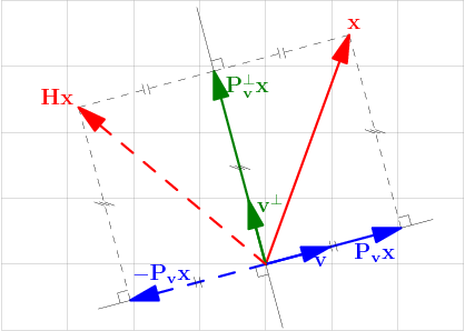
from wikipedia
\[ \begin{aligned} \mathbf {b} - 2 \operatorname {proj} _{\mathbf {u} }\mathbf {b} {} &= \mathbf {b} - 2 {\frac {\left\langle \mathbf {u} ,\mathbf {b} \right\rangle }{\left\langle \mathbf {u} ,\mathbf {u} \right\rangle }}{\mathbf {u} } \\ &= \mathbf {b} - 2 {\frac { \mathbf {u}\cdot \mathbf {u}^T }{\mathbf {u}^T \cdot \mathbf {u} }} \mathbf{b}\\ &= ( I - 2 {\frac { \mathbf {u}\cdot \mathbf {u}^T }{\mathbf {u}^T \cdot \mathbf {u} })} \mathbf{b}\\ &= H_u\mathbf{b} \end{aligned} \]
我们有反射矩阵:
\[ H_u = I - 2 {\frac { \mathbf {u}\cdot \mathbf {u}^T }{\mathbf {u}^T \cdot \mathbf {u} } } \]
为什么要引入这个反射矩阵?
wikipedia 上有关于这个矩阵的说法:
豪斯霍尔德变换可以将向量的某些元素置零,同时保持该向量的范数不变。
将非零列向量 \(\mathbf{x}=[x_1,\ldots,x_n ]^T\) 变换为单位基向量\(\mathbf{e}=[1,0,\ldots,0]^T\) 的豪斯霍尔德矩阵为
\(\mathbf{H} = \mathbf{I} - \frac{2}{\langle \mathbf{v},\mathbf{v} \rangle}\mathbf{vv}^H\)
其中豪斯霍尔德向量\(\mathbf{v}\)满足:
\(\mathbf{v} = \mathbf{x} + \rm{sign}(x_1) \Vert x \Vert_2 \mathbf{e}_1 . \,\)
这个矩阵有特性包括:
- \(H^{T}=H\)
- \(H^{-1}=H\)
- \(H^{2}=I\)
假设 \(\mathbf{a}\) 是矩阵 A 的第一列, 有 \(H_u\) :
\[ c\mathbf{e}_1 = H_u \mathbf{a} \]
也就做完这个操作可做到:
\[ \begin{pmatrix} x & x & x & x\\ x & x & x & x\\ x & x & x & x\\ x & x & x & x \end{pmatrix} \to \begin{pmatrix} 1 & x & x & x\\ 0 & x & x & x\\ 0 & x & x & x\\ 0 & x & x & x \end{pmatrix} \]
这就是我们高斯消元法做的第一步,这也是让我们朝着上三角迈进的第一步。 我们可以继续执行,最终我们可以得到上三角矩阵:
\[ R = H_{u_n} \cdots H_{u_1}A \\ Q = H_{u_1}^T \cdots H_{u_n}^T \]
Gram-Schmidt 和 Householder 对于 \(A^{m \times n}\) 分解会有稍许不同:
- Gram-Schmidt : \(Q \in R^{m \times n}, R \in R^{n \times n}\)
- Householder: \(Q \in R^{m \times m}, R \in R^{m \times n}\)
在计算中,Householder 的数值稳定性会稍优于 Gram-Schmidt.
3.3 计算
\[ A={\begin{pmatrix}12&-51&4\\6&167&-68\\-4&24&-41\end{pmatrix}} \]
\[ Q={\begin{pmatrix}0.8571&-0.3943&0.3314\\0.4286&0.9029&-0.0343\\-0.2857&0.1714&0.9429\end{pmatrix}}\]
\[ R= \begin{pmatrix}14&21&-14\\0&175&-70\\0&0&-35\end{pmatrix} \]
同样,QR 分解直接 scipy.linalg.qr:
import numpy as np
from scipy import linalg

a = np.array([[12, -51, 4],
              [6, 167, -68],
              [-4, 24, -41]])

q, r = linalg.qr(a)

q
# array([[-0.85714286,  0.39428571,  0.33142857],
#       [-0.42857143, -0.90285714, -0.03428571],
#       [ 0.28571429, -0.17142857,  0.94285714]])

r
# array([[ -14.,  -21.,   14.],
#       [   0., -175.,   70.],
#       [   0.,    0.,  -35.]])

np.allclose(np.dot(q, r), a) # True
符号不一样仅仅只是我们基 \(\mathbf{e}_1\cdots \mathbf{e}_n\) 的方向选择.
A = QR 的抗干扰性总觉得不是很好,即使A只有微小的变化,QR 也会剧烈改变。